Annex 8 - Safety Validation of Complex Components - Validation by Analysis
Final Report of WP3.1
European Project STSARCES
Contract SMT 4CT97-2191
Abstract
The aim of the safety validation process is to prove that the product meets the safety requirements. Safety validation of complex programmable systems has become an increasingly common procedure since programmable systems have turned out to be useful also in safety related systems. However, a new kind of thinking related to the whole life cycle of the programmable product is needed and new validation methods (analysis and testing) to support the old methods are inevitable. This means that methods such as failure mode and effect analysis (FMEA) are still applicable, but they are not sufficient. Methods are needed also to guarantee the quality of the hardware and software.
The main validation methods are analysis and tests, and usually both are needed to complete the validation process. Analysis is very effective tool to validate simple systems thoroughly, but a complete analysis can be ineffective against failures of modern programmable electronics. Large programmable systems can be so complicated that a certain strategy in the validation process is necessary to keep the resources required reasonable. A good strategy is to start as early as possible and at the top level (system level). It is then possible to determine the safety critical parts by considering the safety requirements, categories (according to EN 954), safety integrity levels (according to IEC 61508), and the structure of the system. The critical parts are typically parts that the system rely on and which have some properties which cannot be seen clearly at the top level.
A newly arising problem is that large programmable systems are becoming difficult to realise and the analysis is often difficult to understand. Figures can often illustrate the results of the analysis better than huge tables. However, there is no all-purpose excellent illustrating method, but the analyser needs to draw figures so that the main subject is well brought out.
Preface
STSARCES, the Standards for Safety Related Complex Electronic Systems project, is funded mainly by the European Commission SMT (Standards, Measurement and Testing) programme (Contract SMT 4CT97-2191). Work package 3.1 is also funded by the Finnish Work Environment Fund, Nordtest, and VTT. The project aim is to support the production of standards for the functional safety sector of control systems in machinery. Some standards are already available and industry and research institutes have their first experiences in how to apply the standards. Harmonisation of methods and some additional guidelines to show how to apply the standards are needed since the methods for treating and validating safety related complex systems are complicated and not particularly detailed. This report introduces the results of work package 3.1: Validation by analysis. The final format of the report was achieved with help, discussions and comments from Jarmo Alanen, Risto Kuivanen, Risto Tiusanen, Marita Hietikko, Risto Tuominen and partners from the consortium.
The following organisations participated in the research programme:
- INERIS (Institut National de l’Environnement Industriel et des Risques, of France)
- BIA (Berufsgenossenschaftliches Institut fur Arbeitssicherheit, of Germany)
- HSE (Health & Safety Executive, of United Kingdom)
- INRS (Institut National de Recherche et de Sécurite, of France)
- VTT (Technical Research Centre, of Finland)
- CETIM (Centre Technique des Industries Mecaniques, of France)
- INSHT (Instituto Nacional de Seguridad e Higiene en el Trabajo, of Spain)
- JAY (Jay Electronique SA, of France)
- SP (Sveriges Provnings – ach Forkningsinstitut, of Sweden)
- TUV (TUV Product Service GMBH, of Germany)
- SICK AG (SICK AG Safety Systems Division, of Germany)
The research programme work-packages were assigned as :
- Work-package 1: Software safety (leader – INRS)
WP 1.1 Software engineering tasks : CASE tools (CETIM)
WP 1.2 Tools for software faults avoidance (INRS)
- Work-package 2 : Hardware safety (leader – BIA)
WP 2.1 Quantitative analysis (BIA)
WP 2.2 Methods for fault detection (SP)
- Work-package 3 : Safety validation of complex components (leader – VTT)
WP 3.1 Validation by analysis (VTT)
WP 3.2 Intercomparison white-box/black-box tests (INSHT)
WP 3.3 Validation tests (TÜV)
- Work-package 4 : Link between the EN 954 and IEC 61508 standards (leader – HSE)
- Work-package 5 : Innovative technologies and designs (leader – INERIS)
Operational partners: Industrial (SICK AG and JAY) and test-houses (INERIS and BIA)
- Work-package 6 : Appendix draft to the EN 954 standard (leader – INERIS)
Operational partners : STSARCES Steering Committee and industrial partners
Contents
1 Introduction
2 VALIDATION PROCESS
2.1 The Need for Validation
2.2 Safety Validation
2.2.1 Validation Planning
2.2.2 Validation
3 SAFETY ISSUES RELATED TO COMPLEX COMPONENTS
3.1 Analysing Strategy
3.2 Complex Modules and Systems
3.2.1 Analysing Strategy for Modules and Systems
3.2.2 Safety Principles of Distributed Systems
3.3 Complex Components
3.3.1 Failure Modes for Complex Components
3.3.3 Safety Aspects
4 METHODS OF ANALYSIS
4.1 Common Analysis Methods
4.1.1 FMEA
4.1.2 FTA
4.2 Illustrating the Results of a Safety Analysis
4.2.1 The Need to Clearly Show the Results of the FMEA
4.2.2 Examples for Illustrating FMEA Results
4.2.3 Conclusions for Methods of Illustration
5 CONCLUSIONS
GLOSSARY
|
Bottom-up method/analysis/
approach
|
The analysis begins with single failures (events) and the consequences are concluded.
|
|
CAN-bus
|
Control area network; communication method which is common in distributed systems, especially, in mobile machines and cars.
|
|
Component level analysis
|
Analysis is made on level in which the smallest parts are components.
|
|
CPU
|
Central processing unit
|
|
FMEA
|
Failure mode and effect analysis
|
|
FTA
|
Fault tree analysis
|
|
Module level analysis
|
Analysis is made on level in which the smallest parts are modules (subsystems).
|
|
SIL
|
Safety integrity level (IEC 61508)
|
|
System level analysis
|
Analysis is made on high level in which the smallest parts are subsystems.
|
|
Top-down method/analysis/
approach
|
The analysis begins with top events and the initiating factors are concluded.
|
1 Introduction
During the 1980’s, it was realised that it was not possible to thoroughly validate complex programmable electronic components and this resulted in complex electronic components not being used in safety critical systems. However, complex components make it possible to economically perform new complex functions without using many extra components, therefore the possibility of using complex programmable components to also perform safety functions increased. The methods for validating complex systems have developed significantly and they still continue to develop, and as a result, there are currently methods to validate control systems that include complex components.
Complicated integrated circuits and programmable circuits are considered as complex components, however, small devices like sensors or motor control units can be called complex components when the observer has a system point of view. The component is usually a part, which is not designed by the system designer and is bought as a whole; therefore, it is the smallest part that the system designer is controlling. This study is considering the analysis of complex components from different points of view and, therefore, the concept of complex components has several meanings.
Complex components within safety related systems are becoming increasingly common. One reason for this trend is that in general, systems are getting more and more complex and the monitoring and safety functions required are also complicated, therefore more complex control systems are required. This results in very complex systems, where the structures and the functions are difficult to understand and it can be a major problem for the validators. Desired features in safety systems are certain levels of redundancy and diversity, but they make the systems even more complex and difficult to thoroughly understand.
Since the components and the systems are complex they tend to include design errors because it is very difficult to verify, analyse, and test the complete system. Another problem is that the exact failure modes of complex components can also be difficult to predict. The question is, ‘can people trust the complex safety systems?’ If a safety function fails it often causes dramatic consequences since people take higher risks when they feel they can trust the safety system, and it is therefore important for safety systems to perform their safety functions reliably. A validation process provides proof that a safety system fulfils its safety requirements. This report gives guidance on one part of the validation process - validation by analysis, and in particular considers, systems including complex components.
Although complex programmable components can be difficult to validate, they make it possible to perform new kinds of safety and monitoring functions, for example, programmable systems can monitor reasonability of inputs and complicated safety limits, whereas normally these functions would be laborious and expensive to perform with hardwired technology. Therefore complex programmable safety related systems are becoming more common in areas where they are economically competitive. The designer has to decide whether he can accept the risks programmable systems bring along whilst also utilising the possibilities they give.
In general, a validation process is made to confirm by examination and provision of objective evidence, that the particular requirements for a specific intended use are fulfilled. When validation is related to the safety-related parts of a control system, the purpose is to determine the level of conformity to their specification within the overall safety requirements specification of the machinery. [prEN 954-2 1999].
Carrying out a validation process can be a laborious task especially for complicated systems, which have got high safety demands. However, although the process can be laborious it is also necessary. Validation is often needed for the following purposes:
- to prove to customers that the product is applicable for the intended purpose,
- to prove to authorities that the product is safe and reliable enough for the intended purpose,
- to prove to the manufacturer that the product is ready for the market,
- to prove the reasons for specific solutions,
- to provide documentation to help with future alterations of the product,
- to prove the quality of the product.
The validation process has been growing to meet the common needs as the technology has developed. Simple systems can be analysed (FMEA) and tested (fault injection) quite thoroughly. Systems with moderate complexity can also be analysed quite thoroughly, but the tests cannot cover the whole system. Very complex systems cannot be completely analysed in detail and thorough tests are also not possible. A number of different methods are needed in the process. Analysis is required in at least the system level and the detailed component level, but also requirements related to different lifecycle phases have to be fulfilled. This means that attributes such as quality control, correct design methods and management become more important since most of the failures or errors are related to these kind of issues.
Confidence is a very important factor related to the validation process. The user of the validation documents has to trust the validation quality, otherwise the validation has no meaning. The validation activities are actually carried out to convince someone that the product is properly designed and manufactured. One way to increase the confidence is to perform the validation process according to existing requirements and guides, and to have objective experts involved in the validation process.
The safety validation process consists of planning and the actual validation. The same process can also be applied for subsystems. A checklist or alternative guide is required in the process to include all the necessary actions for the safety validation plan.
The phases of the validation process are presented in
figure 1
. First, the validation plan is made according to known validation principles. Then the system is analysed according to the validation plan, the known criteria, and the design considerations. Testing is carried out according to the validation plan and the results of the analysis. All the phases have to be recorded in order to have reliable proof of the validation process and the documents to help future modifications.

Figure 1 Overview of the validation process [prEN 954-2 1999].
When following the figure it is possible to go back from one state to earlier state.
The purpose of safety validation planning is to ensure that a plan is in place for the testing and analysis of the safety requirements (e.g. standards EN 954 or IEC 61508). Safety validation planning is also performed to facilitate and enhance the quality of safety validation. The planning shows the organisation and states in chronological order, the tests and verification activities needed in the validation process. A checklist is needed in the planning process in order to include all the essential analyses and tests into the safety validation plan. Such a checklist can be gathered from IEC 61508-1, prEN 954-2 or the Nordtest Method [Hérard et. al. 1999]. Large control systems may include separate subsystems, which are convenient to validate separately.
The main inputs for safety validation planning are the safety requirements. Each requirement shall be tested in the validation process and the passing criteria shall be declared in the plan. It is also important to declare the person(s) who makes the decisions if something unexpected happens, or who has the competence to do the validation. As a result, safety validation planning provides a guideline on how to perform safety validation.
The purpose of safety validation is to check that all safety related parts of the system meet the specification for safety requirements. Safety validation is carried out according to the safety validation plan. As a result of the safety validation, it is possible to see that the safety related system meets the safety requirements since all the safety requirements are validated. When discrepancies occur between expected and actual results it has to be decided whether to issue a request to change the system, or the specifications and possible applications. Also, it has to be decided whether to continue and make the needed changes later, or to make changes immediately and start the validation process in an earlier phase.
The traditional way to analyse an electronic control system is to apply a bottom-up approach by using Failure Mode and Effect Analysis (FMEA, see 4.1.1). The method is effective and it reveals random failures well. The method is good for systems, which can be analysed thoroughly. Systems are, however, getting more complex and so the top-down approach is getting more and more applicable. A top-down approach like Fault Tree Analysis (FTA, see 4.1.2) helps to understand the system better and systematic failures can also be better revealed. The top-down approach also reveals well failures other than just random failures, which are better revealed by the bottom-up approach.
Another development due to increasing system complexity has been analysis on a module by module basis rather than on a component by component basis. Non-programmable electronic systems with moderate complexity can and should be analysed on a component by component basis and, in some cases (large systems), also on a module by module basis to cover complicated module/system level errors. To analyse complex programmable systems at the component by component basis by using bottom-up analysis (FMEA) would require a lot of resources and yet the method is not the best way to find certain failures. The system functions can be better understood at a module or system level than at a component level and so the quality of the analysis can be improved in that part.
The system analysis could be started from the bottom (not preferable) so that first each of the small subsystems are analysed and finally the system as a whole. In the so-called V-model, the system is designed from the top to the bottom (finest details) and then validated from the bottom to the top. The analysis should, however, be made as soon as possible during the design process in order to minimise possible corrections. Thereby the system should be analysed by starting from the top at system/module level. Then detailed component level analysis can be made in modules which were found critical at module level analysis. This method reduces the resources needed in the analysis. Table 1 illustrates the analysis activities at different levels.
Table
1 System, module and component level analysis and some aspects related to bottom-up analysis and top-down analysis.
|
System level
|
· Bottom-up analysis (e.g. FMEA) is useful and it reveals random failures well.
· Top-down method (e.g. FTA) illustrates the failures well, reveals sequential failures and human errors. Useful when the amount of top events is small.
· At system level (without details) the analysis can often be made thoroughly.
· Validated modules can be used to ease the analysis.
|
|
Module level
|
· Bottom-up analysis is useful and it reveals random failures well.
· Top-down method illustrates the failures well, reveals sequential failures and human errors. Useful when the amount of top events is small.
· Some hints for analysing standardised systems can be found.
|
|
Component level
|
· Bottom-up analysis can be laborious, but necessary for analysing low complexity systems and systems with high safety demands.
· Top-down method or a mixture of top-down and bottom-up methods can be reasonable for analysing complex components, or systems with complex components.
· Usually the system cannot be analysed thoroughly at system level.
|
The common analysing strategy is bottom-up analysis on different levels, but it has some weak points, which have to be taken care of separately. The basic idea in FMEA is to analyse the system so that only one failure is considered at a time. However, common cause failures can break all similar or related components at the same time, especially if there is a miscalculation in dimensioning. These kind of failures have to be considered separately and then added to the analysis. If the safety demands are high, also sequential failures have to be considered carefully since FMEA does not urge the analyser to do so.
More and more often the bottom-up analysis tends to become too massive and laborious, so tactics are needed to minimise the work and amount of documentation. One strategy can be to document only critical failures. Another strategy can be to start the analysis on the most questionable (likely to be critical) structure and then just initially document the items and effects; the failure modes and other information are added only to critical failures. The FMEA table may then look rather empty, but it results in less work.
Many complex components are at the present time too complex to be validated thoroughly (with reasonable resources) and programmable components are becoming even more complicated and specially tailored (e.g. ASIC, FPGA). This means that, for safety purposes, the systems including complex components have to cope with faults by being fault tolerant or by activating automatic safety functions; this can be achieved by concentrating on the architecture. Architecture can be best understood on a system/module level and, therefore, architectural weaknesses can also be conveniently revealed through a system or module level analysis . Additionally, on complex systems there are nearly always some design errors (hardware or software), which can be difficult to find at component level. At module level the analysis can be made thoroughly. One factor supporting module level analysis is the quality of the analysis. An increasing number of components in a unit to be validated corresponds to a reduction in the efficiency of the analysis. Although module level analysis is becoming more and more important, one cannot neglect the analysis at component level because certain failures can be better seen at the component level. A resource saving strategy is to concentrate on critical failures at all levels of analysis. The category (according to EN 954) or the SIL (according to IEC 61508) affects the detail to which the analysis should be performed.
Usually both system/module level and component level analyses are needed in validating complex systems. Analyses on system/module level are performed in order to determine the critical parts of the system, and component level analyses are carried out for those parts of the system.
For module level analysis there are some references which give hints for failure modes of modules and for some standardised systems some advice for analysis can be found, CAN-bus is considered in appendix A as an example. For system/module level analysis, failure modes resemble failures at component level, however, the analyser has to consider the relevant failure modes.
Distributed systems are increasingly used in machinery. Distribution is normally realised by having multiple intelligent modules on a small area communication network. Each module may have several sensor inputs and actuator outputs. The trend, however, is to implement distributed systems with even smaller granularity, i.e. to have a network interface on single sensors or actuators.
Distribution helps to understand and grasp large systems better as the amount of wire is reduced
[1] and the structure of the cabling is more comprehensible. Therefore, the number of mounting faults in a large system is most probably lower compared to a traditional centralised system. Hence, in regard to understandability and cabling simplicity, distributed systems introduce inherent dependability to some extent. Furthermore, in distributed systems it is easier to implement elaborate and localised diagnostic facilities as the system consists of several CPUs capable of doing both off-line and on-line monitoring and diagnostics
[2] The modularity of a distributed system also gives possibilities to implement 'limb home' capabilities in case of a failure in part of the system. These inherent characteristics of distributed systems increase the dependability of the system and therefore also affect the safety of the system in a positive way. However, distributed systems are always complex and hence bring along new kinds of safety problems and aspects, like:
- communication sub-system faults and errors (faults in cables, connectors, joints, transceivers, protocol chips or in the communication sub-system software; transient communication errors)
- communication sub-system design failures (like excessive communication delays, priority inversion and 'babbling idiot')
- system design failures (like scheduling errors or the nodes in the system may have a different view of time of the system state or of the state variables)
When designing distributed systems and busses, various safety techniques can be used to achieve the required safety and dependability level. There is not one ideal solution for all applications.
The analysing strategy described in section 3.1 can also be applied to complex components including distributed systems. In addition to this, distributed systems may have several architectural safety features and techniques for detection, avoidance and control of failures. Such safety principles are described in sections 3.2.2.1 and 3.2.2.2.
Architectural principles crucially affect the safety performance of a safety critical distributed system. There are already some safety-validated busses, which are used for safety critical communication, and such systems always have redundancy and component monitoring. All fieldbusses have some kind of signal monitoring to reveal most of the errors in messages. In some cases the bus standard forces the use of certain architectural solutions. However, on higher level there are more architectural alternatives since large systems may have several different busses that are all used for adequate signalling. This section lists several architectural safety principles or techniques for distributed systems, and brings out the aim and description of each safety technique.
The architectural principles also have to be taken into account during the validation process. Distributed systems are so complex that many kinds of undetected component failures are possible. This means that the architecture of the system has to support fault tolerance and provide a way to force the system into a safe state in case of a failure. Table 2 lists some architectural principles, which should be considered both in the design and validation processes.
Table 2. Architectural principles.
|
Method
|
Applicability
|
|
Hardware topology
|
Hardware topology affects the safe performance of the system. It should be chosen so that in the weakest point the consequences are minimised.
- Redundant hardware topology detects failures by comparing signals between busses (See IEC 61508-7, A.7.3)
- Star topology can operate even if one node is faulty except if it is the node in the star point
- Ring topology can operate even if there is a failure between two nodes [Kuntz, W et al. 1993]
- Redundant ring topology can operate in case of multiple failures in the communication system [Kuntz, W et al. 1993]
- Power supply cabling star topology can supply power from the power source to other nodes even if one node fails or it’s power cables break- provided that each node is fused separately.
|
|
Galvanic isolation [DeviceNet specification]
|
Galvanic isolation prevents different potential levels on distinct nodes to cause unwanted currents between the nodes.
- The communication lines and power supplies of the nodes are galvanically isolated with the help of optoisolators and DC/DC converters.
|
|
Use of a dead man switch line among the bus cables [M3S Specification]
|
Dead man switch provides information to all nodes that the operator of the machine or vehicle is still controlling the system.
|
|
Use of power up/down line among bus cables [M3S Specification]
|
Use of a power up/down line gives a power up signal to all the nodes simultaneously and a power down signal in the case of power down or in an emergency.
- A single wire passing power up/down information is included in the bus cabling and connectors. A total break in the bus cable should correspond to the situation that the power down signal is active.
|
|
Single wire communication [Pers 1992]
|
Single wire communication offers capability to communicate with single wire in case of malfunction in the other wire when twisted pair communication is used.
- With the help of special transceiver circuitry communication can be continued with reduced signal-to-noise ratio in case of interrupt or short in the other twisted pair wire.
|
|
Redundant nodes [Kopetz 1994]
|
Redundant nodes enable continuous operation in the case of a node failure.
- Safety relevant nodes may be replicated to provide a backup node in the case of a failure, which may lead to an accident.
|
|
Global clock [Gregeleit et al. 1994]
|
Global clock provides consistent view of time on all nodes.
- All the nodes of the system should keep an accurate copy of the system time in order to be able to perform time-synchronised operation.
|
|
Shadow node [Kopetz 1994]
|
Shadow node provides a backup for services required in the system.
|
|
Time triggered communication system
[Kopetz 1994]
[Lawson et al. 1992]
|
Assures timeliness of state variables.
-
To implement hard real-time control systems, an event based communication system may not be adequate to guarantee the timeliness of the state variables. In the time triggered approach, communication is scheduled in the design phase of the system prior to the operation. All activities on the bus as well as on the nodes are triggered by time not by events. Hence, the system is predictable and not controlled by stochastic events.
|
This section includes several failure detection, avoidance and control techniques for distributed systems (Table 3). The aims and the main features of each technique are brought out. When the person who analyses the distributed system recognises any of the safety techniques concerning failure detection, avoidance or control, he should observe, what the capabilities of each technique are in order to enhance the safety of the system.
Table 3. Failure detection, avoidance and control techniques.
|
Method
|
Applicability
|
|
Cyclic Redundancy Check (CRC)
|
Errors in received data can be detected by applying CRC over the transferred data.
- The transmitter appends a CRC code to the end of the data frame. The receiver should get the same CRC value as a result when applying the same CRC algorithm (polynomial) to the data of the frame. If the CRC value calculated by the receiver differs from that of the one received in the transmitted frame, the data is regarded as erroneous.
|
|
Communication error recovery by retransmission [Kopetz 1994]
[ISO 11898]
|
Retransmission ensures reliable transfer of data in case of transient failures during transmission.
Messages that are discarded by some of the nodes are retransmitted.
Note! This may cause non-deterministic communication latencies if there is no way to control the retransmission process.
|
|
Message replication without hardware redundancy [Kopetz 1989] (see also IEC 61508-7, A.7.6)
|
Replicating the message by sending it twice or more allows loss of N-1 messages if the message is sent N times.
- Always sending the message twice or more sequentially over a single bus allows deterministic timing compared to that of retransmission in case of failure. If the message is sent twice and the receiver receives the two messages but with different data, both messages must be discarded. If the number of replicated messages is for example three, 2 out of 3 voting can be used.
|
|
Monitoring shorts or open circuits of the bus wires [Pers 1992], [Tanaka et al. 1991]
|
Monitoring shorts or open circuits activates corrective or safety functions in case of a total communication blackout.
- The bus wires are monitored by hardware and signalled to software in case of a malfunction.
|
|
Monitoring bus load [DIN 9684 Teil 3 ]
|
Monitoring bus load enables bus traffic to be restricted dynamically in case of excessive bus load.
- The message rate is monitored by software and if the rate is too high, the nodes are forced to apply inhibit times in their transmission processes.
|
|
Monitoring presence of relevant nodes [CiA/DS301 1999]
|
Monitoring presence of relevant nodes expose accidental drop-out of a node.
Some of the nodes or all nodes monitor the presence of relevant nodes with the help of periodic messages.
|
|
Restricting transmission period of messages [DIN 9684 Teil 3 ]
|
Restricting transmission period disables excessive bus load and thus guarantees proper message latencies for all messages.
- All the nodes of the system are forced to apply specific transmission rate rules in their transmission processes.
|
|
Babbling idiot avoidance [Tindel et al. 1995]
|
Babbling idiot avoidance prevents a single or several nodes from sending erroneously a lot of (high priority) messages, thus gaining exclusive bus access.
|
|
Priority inversion avoidance
|
Messages are controlled so that a low priority message cannot prevent a high priority message from entering the bus.
- This type of situation occurs locally on a node if a low priority message enters the bus contest first and blocks the higher priority message. The situation can be avoided by software and sophisticated hardware, or by time triggered message scheduling.
|
|
Message scheduling based on inhibit times [Fredriksson 1995]
|
Message scheduling based on inhibit times ensures timeliness of the relevant messages on the communication bus.
|
|
Time synchronisation [Fredriksson 1995], [Lawson et al. 1992]
[Kopetz 1994]
|
Time synchronisation ensures timeliness of all the messages on the communication bus.
- Messages are scheduled by synchronising the transmission of a message with respect to time.
|
|
Time stamping
|
Time stamping enables the evaluation of the validity of the data or helps to recognise varying communication delays.
- The arrival time of a message is stored.
|
|
Consistency control of state variables [ISO 11898]
|
Consistency control of state variables ensures that there is no discrepancy between data (and system state) on different nodes.
- The communication protocol should be such that all the nodes accept the correct data from the bus at the same time. If one of the nodes receives incorrect data, all the nodes should discard the data.
|
|
Configuration check
|
Configuration check ensures that correct hardware and software versions are used on the nodes of the system.
- A single node (master) or multiple nodes may check in start-up, with a help of a request message, if the relevant nodes use the presumed hardware and software and parameter versions.
|
|
End-to-end CRC [Kopetz 1994]
|
End-to-end CRC can be used to detect data errors beyond bus communication errors
- Normal CRC checks the data integrity between message transmission and receiving, but the end-to-end CRC also checks data integrity from sensor measurement to message transmission and from message arrival to actuation.
|
|
Message numbering
|
Message numbering ensures correct assembly of the received stream of segmented data or enables discarding of duplicated messages.
- Consecutive messages are numbered, in order to be able to detect discontinuities in the data block or replication of data segments. Numbering can often be accomplished only with a single bit (toggle bit).
|
Complex components hold more than 1000 gates and/or more than 24 pins [EN 954-2 1999]. The definition only provides a rough estimate as to which component could be complex. The amount of potentially different random failures in such a component is large. Only the number of combinations two out of 24 is 276 and this is just the amount of simple short circuits in a small (according to the definition) complex component. Complex components have several failure modes. If one blindly analyses all combinations then this would result in many irrelevant failures. Failure exclusions are needed in order to focus the resources on the critical failures.
Table 4 shows the random failures of the complex components according to prEN 954-2. The table clearly shows all failures related to the input or output of the circuit. The exclusions column shows if it is possible to ignore certain type of failures; so “No” means that the failure mode has to be considered in all cases.
Table 4. Faults to be considered with programmable or complex integrated circuits. [prEN 954-2]
|
Faults considered
|
Exclusions
|
|
Faults of part or all of the function (see a and b)
The fault may be static, change the logic, be dependent on bit sequences
|
No (see a)
|
|
Open-circuit of each individual connection
|
No
|
|
Short circuit between any two connections (see c)
|
No
|
|
Stuck-at-fault; static ”0” and ”1” signal at all inputs and outputs either individually or simultaneously (see c and d)
|
No
|
|
Parasitic oscillation of outputs (see e)
|
No
A fault exclusion can be justified, if such an oscillation cannot be simulated by realistic parasitic feedback (capacitors and resistors).
|
|
Changing value (e.g. in/output voltage of analogue devices)
|
No
|
|
Undetected faults in the hardware which are unnoticed because of the complexity of the integrated circuit (see a and b)
|
No
|
|
Remarks
a - Faults in memory circuits and processors shall be avoided by self-tests, e.g. ROM-tests, RAM-tests, CPU-tests, external watchdog timers and the complete structure of the safety related parts of the control system.
b - The faults considered give only a general indication for the validation of programmable or complex integrated circuits
c - Because of the assumed short-circuits in an integrated circuit, safety signals need to be processed in different integrated circuits separated when redundancy is used.
d - i.e. short circuit to 1 and 0 with isolated input or disconnected output.
e - Frequency and the pulse duty factor dependent on the switching technology and the external circuitry. When testing, the driving stages in question are disconnected
|
However, the basic failures to be considered in the analysis can be simple compared to the actual failures that can happen inside the component. Such component specific failures can for example be, a failure in the microprocessor register or a failure in a certain memory location.
In the draft IEC 61508-2, failures typical to certain component technology (e.g. CPU, memory, bus) are considered instead of the pins (input, output etc.) of the component. A single component can include several technologies.
Table 5 shows some component dependent failures. The table is gathered from draft IEC 61508-2 and the listed failure modes need to be considered when the diagnostic coverage is high
[3]
.
Table 5. Faults or failures of complex components
|
Component
|
Faults or failures to be detected
|
|
CPU
|
|
|
|
Stuck-at faults, stuck-open, open or high impedance outputs, short-circuits between signal lines- all these for data and addresses;
dynamic cross-over for memory cells;
no wrong or multiple addressing
|
- coding and execution including flag register
|
no definite failure assumption;
|
|
|
no definite failure assumption;
|
- program counter, stack pointer
|
Stuck-at faults, stuck-open, open or high impedance outputs, short-circuits between signal lines.
|
|
Bus
|
|
|
|
time out;
|
|
|
wrong address decoding;
|
|
|
all faults which affect data in the memory; wrong data or addresses; wrong access time;
|
|
|
no or continuous or wrong arbitration.
|
|
Interrupt handling
|
no or continuous interrupts;
cross-over of interrupts.
|
|
Clock (Quartz)
|
sub- or superharmonic.
|
|
Invariable memory
|
all faults which affect data in the memory.
|
|
Variable memory
|
Stuck-at faults, stuck-open, open or high impedance outputs, short-circuits between signal lines - all these for data and addresses; dynamic cross-over for memory cells;
no wrong or multiple addressing.
|
|
Discrete hardware
|
|
|
|
Stuck-at faults, stuck-open, open or high impedance outputs, short-circuits between signal lines;
drift and oscillation.
|
|
|
Stuck-at faults, stuck-open, open or high impedance outputs, short-circuits between signal lines;
drift and oscillation.
|
|
|
Stuck-at faults, stuck-open, open or high impedance outputs, short-circuits between signal lines;
drift and oscillation.
|
|
Communication and mass storage
|
all faults which affect data in the memory;
wrong data or addresses; wrong transmission time;
wrong transmission sequence.
|
|
Electromechanical devices
|
does not energise or de-energise; individual contacts welded, no positive guidance of contacts, no positive opening.
|
|
Sensors
|
Stuck-at faults, stuck-open, open or high impedance outputs, short-circuits between signal lines;
drift and oscillation.
|
|
Final elements
|
Stuck-at faults, stuck-open, open or high impedance outputs, short-circuits between signal lines;
drift and oscillation.
|
|
a - Bus-arbitration is the mechanism for deciding which device has control of the bus.
b - "stuck-at" is a fault category which can be described with continuous " 0" or " 1" or "on" at the pins of a component.
|
It is obvious that the person validating the system has to decide which possible failures have to be documented. Usually an expert can see from the circuit diagram which failures can cause severe effects, but generic rules how to neglect some failures can be hard to find. For some standardised technologies it is possible to find in advance the critical failures to consider. This minimises the amount of failures to be considered, and improves the quality of the analysis.
Systematic failures related to complex components and complex systems become even more obvious. There are errors in most commercial programs (usually more than 1/1000 code lines), but usually the errors appear relatively seldomly [Gibbs 1994]. Hardware design failures are probable in complex components and especially in tailored components. Consequently, in complex systems, systematic errors are more common than random failures. The whole system has to be validated and both systematic and random failures have to be considered.
Appendix A shows as an example what kind of failures are related to CAN-bus. Most of the described failures can be used with other types of distributed systems, but the analyser has to know the special features related to the system that is under consideration.
Different analysing techniques are needed in different phases of the design. At first, hazard identification and risk analysis techniques are useful, for example techniques such as, “Hazard and Operability study (HAZOP)”, “Preliminary Hazard Analysis (PHA)”, and techniques which use hazard lists. There are many techniques for software verification and for probabilistic approach to determine safety integrity. In software verification the software errors are searched systematically by using for example data flow analysis, control flow analysis, software FMEA, or sneak circuit analysis (see IEC 61508-7). In probabilistic approach, it is expected that the verification process has already been carried out, and statistical values are used to calculate a probabilistic value for executing the program correctly. There are also methods for verifying components, such as ASIC, designs. This chapter, however, is concentrating on analysis techniques which are used in analysing control systems.
There are two basic types of techniques for analysing systems:
- Top-down methods (deductive), which begin with defined system level top event(s) and the initiating factors are concluded.
- Bottom-up methods, which begin with single failures and the system level consequences are concluded.
Both analysing techniques have their advantages and disadvantages, but ultimately the value of the results depend on the analyst. The techniques can, however, make the analyst more observant to detect certain type of failures or events. Bottom-up methods tend to help the analyst to detect all single failures and events, since all basic events are considered. Top-down methods tend to help the analyst to detect how combined effects or failures can cause a certain top event. Top-down methods are good only if the critical events have to be analysed. Bottom-up methods are good if the whole system has to be analysed systematically. The basic demand is that the analysing technique must be chosen so that all critical events are to be detected with the minimum duty. Top-down methods give an overview of the system, show the critical parts, systematic failures and human factors. Bottom-up methods consider the system systematically and many failures are found.
A combined bottom-up and top-down approach is often likely to be an efficient technique. The top-down analysis provides the global picture and can focus the analysis to areas that are most significant from the overall performance point of view. Bottom-up methods can then be focused on the most critical parts. Bottom-up analysis aims at finding ”the devil that hides in the details”.
The most important point after choosing the analysing method is to concentrate on the weak points of the method, and this can be done by using strict discipline. The weak points of FMEA and FTA are described in chapters 4.1.1 and 4.1.2.
When the safety and performance of a control system is assessed, the Failure Mode and Effect Analysis (FMEA) is the most common tool used. An international standard (IEC 812. 1985) exists to defines the method. FMEA is a bottom-up (inductive) method, which begins with single failures, and then the causes and consequences of the failure are considered. In the FMEA, all components, elements or subsystems of the system under control are listed. FMEA can be done on different levels and in different phases of the design which affects the depth of the analysis. In an early phase of the design, a detailed analysis cannot be done, and also some parts of the system can be considered so clear and harmless that deep analysis is not seen as necessary. However, in the critical parts, the analysis needs to be deep and it should be made on a component level. If the safety of the system really depends on a certain complex component, the analysis may even include some inner parts of the component, for example this can mean software analysis or consideration of typical failures related to a certain logical function.
In prEN 954-2 there are useful lists for FMEA on failures of common components in different types of control systems. The standard gives probable component failures and the analyst decides if the failures are valid in the system considered or if there are other possible failures. If functional blocks, hybrid circuits or integrated circuits are analysed then the list in prEN 954-2 is not enough. Additionally, systematic failures and failures typical to the technology (microprocessors, memories, communication circuits etc.) have to be considered since those failures are more common than basic random hardware failures.
FMEA is intended mainly for single random failures and so it has the following weak points:
- It does not support detection of common cause failures and design failures (systematic failures).
- Human errors are usually left out; the method concentrates on components and not the process events. A sequence of actions causing a certain hazard are difficult to detect.
- Sequential failures causing a hazard can also be difficult to detect, since the basic idea of the method is to consider one failure at a time. If the analysis is made with strict discipline it is also possible to detect sequential failures. If a failure is not detected by the control system, other failures (or events) are studied assuming the undetected failure has happened.
- Systems with a lot of redundancy can be difficult to consider since sequential failures can be important.
- The method treats failures equally, and so even failures with very low probability are considered carefully. This may increase the workload and cause a lot of paper-work.
- In a large analysis documentation, it can be difficult to identify the critical failures. It can be difficult to see which failures have to be considered first, and what the best means are to take care of the critical failures.
However, FMEA is probably the best method to detect random hardware failures, since it considers all components (individually or as blocks) systematically. Some critical parts can be analysed on a detailed level and some on a system level. If the method seems to become too laborious, the analysis can be done on a higher level, which may increase the risk that some failure effects are not detected.
The FMEA table always includes the failure modes of each component and the effects of each failure mode. Since the analysis is carried out to improve the system or to show that the system is safe or reliable enough, some remarks and future actions are also always needed in the table. Severity ranking is needed to ease the comparison between failure modes, and therefore it helps to rank the improvement actions. When the analysis includes criticality ranking it is called Failure Mode, Effects, and Criticality Analysis (FMECA). The criticality and probability factor can be a general category, like; impossible, improbable, occasional, probable, frequent, or exact failure probability values can be used. In many cases exact values are not available because they are difficult to get, or they are difficult to estimate. The circumstances very much affect the probability of a failure.
Table 6 shows an example of a FMECA sheet.
Table 6. Example sheet of a FMECA table (see figure 2).
|
Safety Engineering
|
FMECA
System: Coffee mill
Subsystem:
|
Page:
Date:
Compiled by:
Approved by:
|
|
Item and function
|
Failure mode
|
Failure cause
|
Failure effects
|
Detection method
|
Probability & Severity
|
Remarks
|
|
Switch
|
Short circuit
|
- Foreign object, animal or liquid
- isolation failure (moisture, dirt, ageing
- bad, loose connection, vibration, temp. changes
- overheating (lack of cooling)
|
a) Coffee mill cannot be stopped by actuating the switch. Someone may cut his finger.
b) When the plug is put in, the coffee mill starts up although the switch is in the off state. Someone may cut their finger.
|
Coffee mill does not stop. Switch may become dark.
|
a) 3C
b) 4C
|
The coffee mill can be stopped by un-plugging it.
|
|
Switch
|
Open circuit
|
- The switch mechanism fails to operate, mechanism jams, breaks
|
The coffee mill cannot start up.
|
|
1D
|
|
Fault Tree Analysis (FTA) is a deductive technique that focuses on one particular accident or top event at a time and provides a method for determining causes of that accident. The purpose of the method is to identify combinations of component failures and human errors that can result in the top event. The fault tree is expressed as a graphic model that displays combinations of component failures and other events that can result in the top event. FTA can begin once the top events of interest have been determined. This may mean preceding use of preliminary hazards analysis (PHA) or some other analysis method.
The advantages of FTA are typically:
- It can reveal single point failures, common cause failures, and multiple failure sequences leading to a common consequence.
- It can reveal when a safe state becomes unsafe.
- The method is well known and standardised.
- The method is suitable for analysing the entire system including hardware, software, any other technologies, events and human actions.
- The method provides a clear linkage between qualitative analysis and the probabilistic assessment.
- It shows clearly the reasons for a hazardous event.
The disadvantages of FTA are typically:
- It may be difficult to identify all hazards, failures and events of a large system.
- The method is not practical on systems with a large number of safety critical failures.
- It is difficult to introduce timing information into fault trees.
- The method can become large and complex [Ippolito & Wallace 1995].
- The method gives a static view to system behaviour.
- The method typically assumes independence of events, although dependencies can be present; this affects the probability calculations. The dependencies also increase the work.
- It is difficult to invent new hazards which the participants of the analysis do not already know.
- Different analysts typically end up with different representations, which can be difficult to compare.
Quite often probability calculations are included in the FTA. FTA can be performed with special computer programs, which easily provide proper documentation. There are also programs, which can switch the method. The analysis only needs to be fed once, and the program shows information in the form of FTA or FMEA. Figure 2. shows an example of one hazardous event in an FTA format. The figure on the right illustrates the system (Hammer 1980, IEC 1025 1990).

Figure 2. Example shows as a fault tree analysis sheet how some basic events or failures can cause one hazardous top event. The analysed coffee mill is introduced on the top right corner [Hammer 1980].
Complex components are increasingly used in circuits and even one complex component can make the system very complicated. Complex components allow functions, which are difficult to implement with traditional electronics, and they also make communication easier. Complex programmable components make it possible to construct large and complicated systems, which are also difficult to analyse.
When the system is large and an analysis is made in the component level, the analysis requires a lot of work and produces a lot of paper. Control systems with complex components are typically large and so the FMEA project is also large. When the analysis is large it is difficult to verify and to take advantage of, the critical events can easily be lost in the huge amount of information, and it is also difficult to find the essential improvement proposals. Therefore a method is required, which has the advantages of the FMEA, but which does not come with the high level of paper-work.
The method needs to be simple since people tend to avoid complicated new methods. Something familiar is also needed so that the results are easy to understand. Quite often when the FMEA is performed the analyst draws his markings on the circuit diagram to help him to understand the functions of the diagram and also to confirm that all parts of the circuit diagram are considered. This kind of method can also be useful for illustrating results of the FMEA. However, since usually the main purpose of the method is to help the analyst, a good discipline is needed to also make the markings readable for other people.
VTT has studied, in parallel with FMEA, some graphical techniques which can express the key results of the FMEA more effectively than text and tables. The analysis of a power distributing system of a large facility is used here as an example. A power failure could cause severe damages in some occasions. Critical failures were found in FMEA, but since FMEA was quite large, i.e. over 200 pages, the key information was lost in the tables. Therefore a technique was needed to point out the essential results of the analysis.
The analysis was carried out in the system level and only some parts were analysed in the component level. Three different techniques were used in illustrating the FMEA results. First, a fault tree analysis format was used for illustrating some top events; next, flux diagrams of the energy flows were used to illustrate the critical paths; finally, a circuit diagram with severity ranking numbers and colours was used to point out the most critical parts of the system. The probability factor was not shown in the figures, but it would not be difficult to add it into the figures. The techniques were only compared in this single example case, but some general results can also be adapted to other systems.
FTA for illustrating FMEA results
Fault tree analysis (FTA) was only carried out for some top events, and the main purpose in this case was to point out the critical failures discovered in the FMEA (Figure 3). Only some top events were studied since the overall number of such events was large. There were several facilities involved and there were also several top events for each facility, and this meant that many figures were needed. Depending on the operating mode some specific failures caused different top events. Since some single failures were needed in several figures the amount of information increased. As a result the amount of information became so large that it was difficult to find the essential information from the FTA figures.
The result was that FTA was not, in this case, a good method for illustrating the FMEA results. FTA is good technique when the number of top events is not large and there are no dependencies between the top events. The advantage of the FTA is that it is a clear, well-known and well-documented technique. There are also software tools available for drawing the fault trees. If the tool can convert (FMEA) tables and (FTA) trees, it is especially useful.

Figure 3. FTA format figure for one top event.
Flux diagrams for illustrating FMEA results
Flux diagrams were drawn to illustrate criticality of the energy flows. Energy flow meant that the power was switched on and the critical function was able to proceed. The diagram was improvised to illustrate the different failure criticality properties of the energy flows. In a flux diagram, different arrows indicated different criticality levels. The same energy flow or facility did not always have the same criticality level, but the criticality did depend on the system operation mode (processing activities with different facilities). Therefore the figures were able to point out the critical failures during a certain operation mode. One operation mode period did last anywhere between a few minutes to a number of weeks. It was important to know the risks during a certain operation mode, and so several diagrams were needed to illustrate the criticality of a specific energy flow or facility. The technique was new and therefore each marking needed explanation. The meanings of the arrows used were not obvious and although there were only approximately six different arrows used, reading the results required some experience. Figure 4 aims to show which functions are needed during a certain operation and the severity of the failure of each energy flow path.
 Figure 4. The flux diagram shows which functions are needed during a certain operation and the criticality of each energy flow path. NA means not applicable and that function is not needed in the illustrated operation.
Circuit diagrams with a ranking system to illustrate FMEA results
The starting point in drawing the circuit diagram with a ranking system was the main circuit diagram of the system. The diagram was redrawn into a file in order to make quick changes easier. Different colours were then used to indicate the criticality of each circuit or equipment. There were five severity levels, but only the three highest levels were assigned a distinct colour as the lowest levels were considered non-significant. For some parts of the system a number was also used, which indicated the severity of failure in power supply. The FMEA did consist of over 200 pages, but the key results could be put into one colourful diagram. The people in the company were familiar with the diagram since it resembled the original system level circuit diagram of the system. In this case “the circuit diagram with a ranking system” technique was quick to use and it was capable of illustrating effectively the key results of the FMEA.
Although the illustration technique was used here for a large system, it can also be useful for smaller systems, especially during the design process. An expert can quickly colour the circuit diagram and add reference numbers (refers to text) and criticality numbers into the diagram. The colours and numbers can be drawn with pencils, but the changes may be messy to accomplish therefore graphic files can be more useful.
Figure 5 shows an example of this simple method. In the figure a high ranking number means high consequence severity and * means that the severity is low (i.e. consequences of failure are insignificant). The numbers are related to a certain operational unit and beside the number is the name of the unit. If there is a shortage of space, reference numbers can be used. The severity of consequences (max.) related to failure of switches or cables is expressed by using different colours.

Figure 5. An example of the circuit diagram representation.
The advantages of the technique are:
- the technique is simple and it is easy to use
- it is easy to improvise new adequate markings
- the technique is quick to use especially when the circuit diagrams are easily available
- the technique shows in a very compact form the risks of the analysed system
- the technique displays well the most critical risks
- electricians feel that the technique is familiar since circuit diagrams are used.
The disadvantages of the diagram are:
- it is hard to introduce new markings and all markings must be explained each time
- people have to learn the technique before it is useful
- the technique is not standardised
- information is lost when it is shrunk into one figure
- the technique can only effectively show single hardware failures
- it is difficult to express events other than failures.
FMEA is a common, reliable, but laborious method to analyse control systems. In large systems the analysis work can be more effective if some other method, or FMEA in a very high level, is used to locate the critical parts of the system. The amount of reasonable effort for analysing a system also depends on safety demands. If safety demands are high, then more effort can be allocated to be sure of the performance of the safety critical functions. Another problem arises when the amount of information in the FMEA is so huge that the essential results are lost. Figure 6 shows how the bottom-up method can be supported by other techniques.

Figure 6. Common methods to support the use of bottom-up analysis. Detailed bottom-up analysis is carried out only to some parts of the system.
It is not always clear how to point out the most essential results of the FMEA. Usually a critical items list and an improvement list is made to demonstrate the results of the analysis, but often a graphical method can show the results better than words. Graphical techniques are very powerful in pointing out certain results, and different graphical techniques provide different points of view of the results, so the analyst must decide which technique best illustrates the essential results. FTA shows well which events or failures may cause a top event. Flux diagrams can effectively show critical paths. Circuit diagrams with ranking information show which parts of the system are the most critical.
No single perfect method exists, which can best illustrate the most critical failures or events; therefore the analyst has to decide on case by case basis which technique to use. Important factors to be considered are:
- type of results; should the results consider failures, events, human errors, and software errors?
- extent of the analysis and resources
- quantity of the results to be illustrated
- audience
- type of figures the audience is familiar with.
In some cases, FMEA is carried out to find a major critical failure, “show stopper”, which ends the analysis, because the system then has to be redesigned and the analysis starts from the beginning. If no critical failure is found then all the documentation is important because it provides a piece of proof for safety. If a critical failure is found, it must be well documented.
There does not exist a single ideal approach to analyse complex systems. However, some guidelines for using top-down analysis like FTA (Fault Tree Analysis) or bottom-up analysis like FMEA (Failure, Mode and Effect Analysis) can be stated. FMEA and FTA are the most common methods for analysing failures of control systems. One reason for selecting a certain method is the common practice. If a person is familiar with a certain method and he can use all the required tools for that method, then the analysis can be performed more effectively than with a new type of analysis method.
Both FTA and FMEA can be used in the system level, module level or component level. The difference between methods appears when certain types of failures are sought. In FTA, good system specialists are essential and the results depend very much on what they can find. Good system specialists can also point out the essential failures and so reduce the resources required for the analysis. In FMEA, it is slightly easier to replace experience with hard work since the system is analysed systematically. FMEA is usually more laborious than FTA, but it can reveal some new random failures. One way to ease the FMEA analysis is to document in the analysis table only the most critical consequences.
In comparison to more simple components, complex components introduce new aspects to be considered. Complex components are indeed so complex that it is difficult to analyse them thoroughly, and it is very difficult to predict the failure modes of the components. Also, the programs related to programmable components may contain critical errors. All these reasons cause some uncertainty related to the analysis of the complex components. A single complex component alone cannot control a safety function safely enough, because some redundancy, diversity and/or monitoring is needed. This means that the architecture of the control system is important and it can make the risks caused by complex components to become negligible.
REFERENCES
CiA/DS301. 1999. CANopen Application Layer and Communication profile V4.0. Nürnberg: CAN in Automation International Users and Manufacturers Group e.V. 111 pages.
DeviceNet specification, release 2. DeviceNet Physical Layer and Media (Layer 1 - Physical Layer), 1997, Open DeviceNet Vendor Association, Inc.
DIN 9684 Teil 3. 1993. Landmaschinen und Traktoren - Schnittstellen zur Signalüberteagung - Initialisierung, Identifier (draft). Berlin: DIN Deutsches Institut für Normung. 28 pages.
EN 954-1. 1996. Safety of machinery – Safety related parts of control systems. Part 1: General principles for design.
Fredriksson, L.-B. 1995. CAN Kingdom. rev. 3.0. Kinnahult: Kvaser AB. 104 pages.
Gibbs, W. 1994. Software’s Chronic Crisis. Scientific American, September 1994. http://www.di.ufpe.br/~java/graduacao/referencias/SciAmSept1994.html
Gregeleit, M. & Streich, M. 1994 Implementing a distributed high-resolution real-time clock using CAN-bus. 1. International CAN Conference Proceedings. Erlangen: CAN in Automation e.V. pp. 9-2 ... 9-7.
Hammer, W. 1980. Product Safety Management and Engineering. Prentice-Hall, Inc., Englewood Cliffs, N.J. 324 p.
Hérard, J., Jacobson, J., Kivipuro, M., Malm, T., Ståhlhane, T. & Tiusanen, R. Guideline for the validation of Functional Safety according to IEC 61508. Proposal for Nordtest Method. 48 p.
Ippolito, L. & Wallace, D. 1995. A study on Hazard Analysis in High Integrity Software Standards and Guidelines. NIST, Gaithersburg, U.S. Department of commerce. http://hissa.ncsl.nist.gov/HHRFdata/Artifacts/ITLdoc/5589/hazard.html#36..., 45 p.
IEC 812. 1985. Analysis techniques for system reliability - Procedure for failure mode and effect analysis (FMEA). International Electrotechnical Commission. 41 p.
IEC 1025. 1990. Fault tree analysis (FTA). International Electrotechnical Commission. 40 p.
IEC 61508 -1 : 1998. Functional safety of electrical/electronic/programmable electronic safety-related systems. Part 1: General requirements
IEC 61508 - 3 : 1998. Functional safety of electrical/electronic/programmable electronic safety-related systems. Part 3: Software requirements.
IEC 61508 - 4 : 1998. Functional safety of electrical/electronic/programmable electronic safety-related systems. Part 4: Definitions and Abbreviations
IEC 61508 - 5 : 1998. Functional safety of electrical/electronic/programmable electronic safety-related systems. Part 5: Guidelines on the application of Part 1.
IEC 65A/254/CDV Draft IEC 61508-2. Functional safety of electrical/ electronic/ programmable electronic safety-related systems. Part 2: Requirements for electrical/ electronic/ programmable electronic safety-related systems
IEC 65A/255/CDV Draft IEC 61508-6. Functional safety of electrical/ electronic/ programmable electronic safety-related systems. Part 6: Guidelines on the application of parts 2 and 3.
IEC 65A/256/CDV Draft IEC 61508-7 Functional safety of electrical/ electronic/ programmable electronic safety-related systems. Part 7: Overview of techniques and measures
ISO 11898. 1993. Road vehicles - Interchange of digital information - Controller area network (CAN) for high-speed communication. International Organization for Standardization (ISO). 58 pages.
Kopetz, H. & Damm, A. & Koza, C. Mulazzani, M. & Schwabl, W. & Senft, C. & Zainlinger, R. 1989. Distributed Fault-Tolerant Real-Time Systems: The Mars Approach. IEEE Micro Feb 1989. Pages 25-40.
Kopetz, H. 1994. Fault Management in the Time Triggered Protocol (TTP). Warrendale: Society of Automotive Engineers (SAE). 7 pages. (SAE paper 940140).
Kuntz, W. & Mores, R. & Morse, M.J. 1993. CAN operated on an optical double ring at improved fault-tolerance. European Transactions on Telecommunications and Related Technologies. Vol. 4, issue 4, pp. 465 - 470. ISSN 1120-3862.
Lawson, H.W. & Lindgren, M. & Strömberg, M. & Lundqvist, T. & Lundbäck, K.-L. & Johansson, L.-Å. & Torin, J. & Gunningberg, P. & Hansson, H. 1992. Gudelines for Basement: A Real-Time Architecture for Automotive Systems. Göteborg: Mecel, Inc. and Lidingö: Lawson Publishing and Consulting, Inc. 42 pages.
Lehtelä, M. 1991. Failure Mode and Effect Analysis of Electronic Circuits. Tampere University of Technology, Electrical Engineering Department. Licentiate thesis. 77 p. + app. 12 p.
M3S Specification 2.0. 1995. An intelligent integrated and modular system for the rehabilitation environment. M3S draft standard, ISO/TC-173/SC-1/WG-7.
Pehrs, J-U. 1992. CAN bus failure management using the P8xC592 microcontroller. Philips Application Note, Report Nr: HKI/AN 91 020. Hamburg: Product Concept & Application Laboratory, 1992. 16 pages.
PrEN 954-2. 1999. Safety of machinery – Safety related parts of control systems. Part 2: Validation.
Tanaka, M. & Hashimoto, K. & Himino, Y. & Suzuki, A. 1991. High-reliability physical layer for in.vehicle high-speed local area network. Warrendale: Society of Automotive Engineers (SAE). 9 pages. (SAE paper 910464).
Tindell, K. & Burns, A. 1994. Guaranteed Message Latencies for Distributed Safety-Critical Hard Real-Time Control Networks. Technical report YCS229. York: University of York. 17 pages.
Tindell, K., Hansson, H. Babbling Idiots, the Dual-Priority Protocol, and Smart CAN Controllers. 2nd International CAN Conference, 1995. pp 7-22 .. 7-28.
APPENDIX A:
CAN bus FMEA
The CAN bus is originally made for road vehicles, but increasingly the system is often used in machine automation. Also some so called “safety busses” are based on CAN.
CAN modules are analysed using FMEA at I/O level. In this case the individual components inside the modules are not analysed. The results would depend on the type of the components and the components are developing rapidly. The FMEA is carried out according to the principles of IEC 812.
During normal operation, several bus failures may occur that could influence the bus operation. These failures and the resulting behaviour of the network are illustrated in Figure A1 and described in table A1. The possible open circuit and short circuit failures are given by the CAN standard [ISO 11898]. The failure 16 is not exactly in the ISO standard, but the failure differs from failure 15 if the shield is grounded from one point. These failure modes should be taken into account in CAN bus FMEA.
 Figure A1. Possible failure modes of bus line according to ISO 11898. Failure modes 10-15 are not numbered in ISO 11898[4] and failure mode 16 is not given in ISO 11898. Failure modes 10-12 are interpreted as a single failure mode in ISO 11898.
Table A1. Bus failure detection according to ISO 11898.
|
Description of bus failures
|
Behaviour of network1)
|
Quality of specification2)
|
|
One node becomes disconnected from the bus (10,11,12)
|
The remaining nodes continue communicating.
|
Recommended.
|
|
One node loses power (13)
|
The remaining nodes continue communicating with reduced signal to noise ratio.
|
Recommended.
|
|
One node loses ground (14)
|
The remaining nodes continue communicating with reduced signal to noise ratio.
|
Recommended.
|
|
The connection to the shield breaks off in any node (15)
|
All nodes continue communicating.
|
Recommended.
|
|
The connection to the shield breaks off and all nodes lose shield connection (16)
|
All nodes continue communicating, but disturbances are more probable.
|
-----
(no reference to ISO 11898)
|
|
CAN_H interrupted (1)
|
All nodes continue communicating with reduced signal to noise ratio.
|
Recommended.
|
|
CAN_L interrupted (2)
|
- ” -
|
Recommended.
|
|
CAN_H shorted to battery voltage (3)
|
- ” -
|
Recommended.
|
|
CAN_L shorted to ground (4)
|
- ” -
|
Recommended.
|
|
CAN_H shorted to ground (5)
|
- ” -
|
Recommended.
|
|
CAN_L shorted to battery voltage (6)
|
- ” -
|
Recommended.
|
|
CAN_L wire shorted to CAN_H-wire (7)
|
- ” -
|
Optional.
|
|
CAN_H and CAN_L wires interrupted at the same location (8)
|
No operation within the complete system. Nodes within the resulting subsystem that contains the termination network contains communication.
|
Recommended.
|
Table A1. Continued
|
Loss of one connection to termination network (9)
|
All nodes continue communicating with reduced signal to noise ratio.
|
Recommended.
|
|
1) The example in figure A1 excludes all fault tolerant modes
2) The quality of specification is defined as follows.
Recommended: If the respective failure occurs the network behaviour should be as described in the second column of the table. To exclude this specified functionality is the manufacturer’s choice.
Optional: If the respective failure occurs the network behaviour may be as described in the second column of the table. To include this fuller specified functionality is the manufacturer’s choice.
|
[1] At least the total length of the wires is reduced, but the number of items (number of wires, connectors or joints, etc.) is not reduced in all cases.
[2] It should, however, be noted that not all diagnostic facilities increase the dependability of the system compared to a less intelligent system; some diagnostic facilities must be implemented only to maintain the same level of dependability as that of the previous generation 'old-fashioned' control systems.
[3] =fractional decrease in the probability of dangerous hardware failure resulting from operation of the automatic diagnostic tests [IEC 61508-4:1998]
[4] Note also that in some editions of the ISO 11898 standard, the numbering of the failure modes is not consistent: the illustrative figure and the detailed table of the ISO standard do not match with the failure mode numbers. The numbering given in Figure A1 follows the numbering of the table in the ISO 11898.

 is defined as follows:
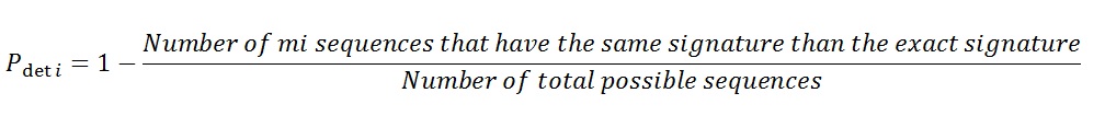

 ,
, 

 erroneous base sequences,
  erroneous sequences by combining base pairs, etc ..., and finally an erroneous sequences by combining all base sequence sequences or
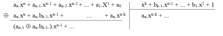
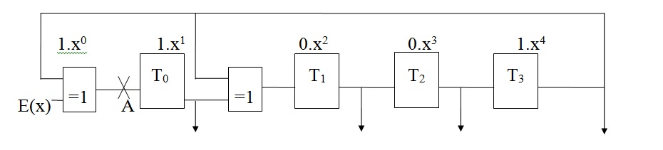
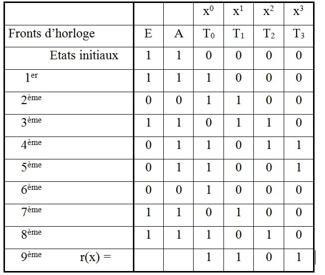
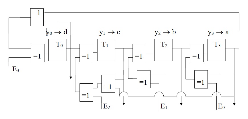
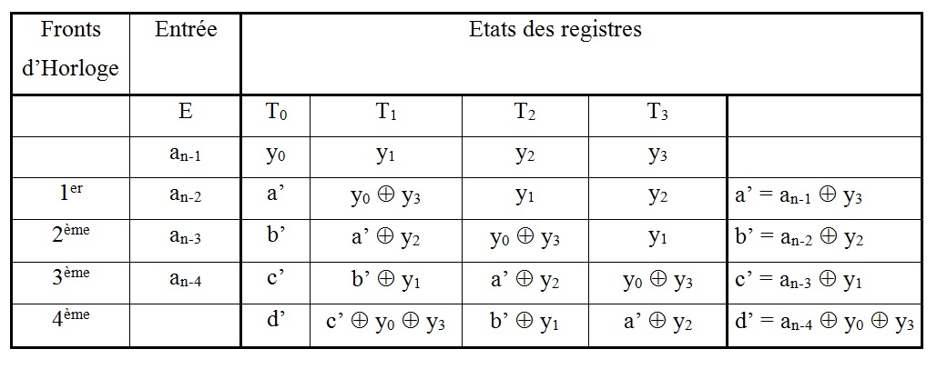
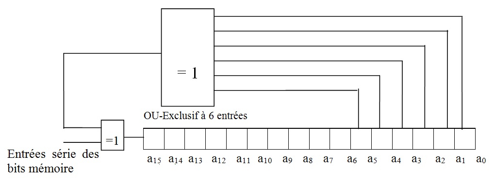
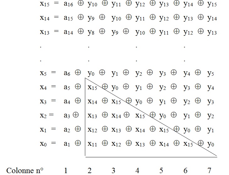


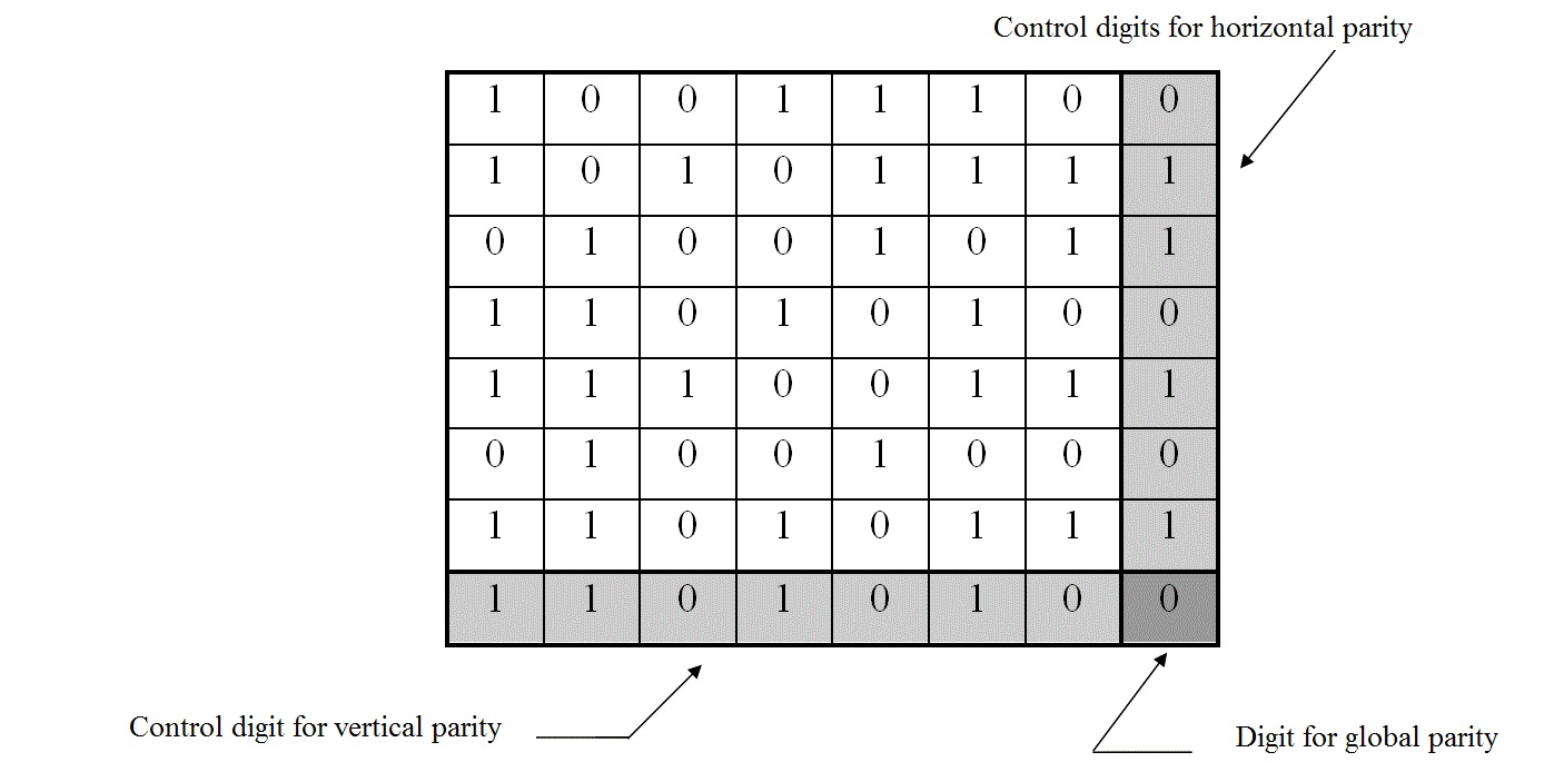

 of combinations of "N" bytes whose sum is identical to the sum "S" obtained on the bytes of the
 ; P = 8 bits (the number of bits in a byte)


 and
and 

 and
and 

 .
.

 d min:
 H errors such that
 .
.


 (
(